
by Olivier Leduc
In the late 80’s, Kearns and Valiant asked the following question:
Can a set of weak learners be used to create a strong learner?
A weak learner is a classifier that can identify the correct label better than randomly guessing would. The question was answered in the positive by Schapire (1990), and implemented, with Freund, in the form of AdaBoost.
While the various No Free Lunch Theorems guarantee that no supervised learning algorithm is always best regardless of context and data, AdaBoost with weak decision tree learners is thought to be the “best out-of-the-box classifier” (Wikipedia).
This idea of grouping weak models to improve the final result was also implemented with… pigeons. Yes, you read that correctly: pigeons. Scientists trained 16 pigeons (weak learners if ever there were ones) to identify pictures of magnified biopsies of possible breast cancers. On average, each pigeon had an accuracy of about 85%, but when the most popular answer among the group was selected, the accuracy jumped to 99% (see https://www.scientificamerican.com/article/using-pigeons-to-diagnose-cancer/ for more details).
The pigeon work above is a form of bootstrap aggregation (also known as bagging). In this article, we present two algorithms that use a different approach to answer Kearns and Valiant’s question: AdaBoost and Gradient Boosting, which are two different implementations of the idea behind boosting.
Table of Contents
AdaBoost
AdaBoost stands for Adaptive Boosting, adapting dynamic boosting to a set of models in order to minimize the error made by the individual models (these models are often weak learners, such as “stubby” trees or “coarse” linear models, but AdaBoost can be used with many other learning algorithms). AdaBoost is adaptive meaning that any new weak learner that is added to the boosted model is modified to improve the predictive power on instances which were “mis-predicted” by the (previously) boosted model. The main idea behind dynamic boosting is to consider a weighted sum of weak learners whose weights are adjusted so that the prediction error is minimized.
In the two-category classification context, for instance, the training data might consist of the following  observations:
  , where
  . The boosted classifier, then, is a function
![\[F({\vec{x})=\sum_{m=1}^Mc_mf_m(\vec{x}),\]](https://www.data-action-lab.com/wp-content/ql-cache/quicklatex.com-dc054cfac6195a8a357bb7f82ab2cb06_l3.png "Rendered by QuickLaTeX.com")
 for all
  and all
  , and
, and  is constant for all . The class prediction at is simply
  . The AdaBoost contribution comes in at the modeling stage, where, for each
  the weak learner
  is trained on a weighted version of the original training data, with observations that are misclassified by the partial boosted model
 ![\[F_{\mu}(\vec{x})=\sum_{m=1}^{\mu-1}c_mf_m(\vec{x})\]](https://www.data-action-lab.com/wp-content/ql-cache/quicklatex.com-6cd5c495accc07b2a8d43a43fcf25f12_l3.png "Rendered by QuickLaTeX.com")
 ,
,  at each of the boosting steps
  .
.
Friedman, Hastie, and Tibshirani (1998) present a generalization of this model (called Real AdaBoost) which does away with the constants  :
:
- Initialize the weights
 , with
  , for
, for  ;
; - For , repeat:
- fit the class probability estimate
 , using the weak learner algorithm of interest;
 - define
 ;
; - set
 , for ;
 - renormalize so that
 ;
;
- fit the class probability estimate
- Output the classifier
 .
.
For regression tasks, this procedure must be modified to some extent (in particular, the equivalent task of assigning larger weights to currently misclassified observations at a given step is to train the model to predict (shrunken) residuals at a given step… more or less).
Since boosting is susceptible to overfitting (unlike bagging and random forests), the optimal number of boosting steps  may be derived from cross-validation.
Implementation
The Python library scikit-learn provides a useful implementation of AdaBoost. In order to use it, a base estimator (that is to say, a week learner) must first be selected. In what follows, we will use a decision tree classifier. Once this is done, a AdaBoostClassifier object is created, to which is fed the weak learner, the number of estimators and the learning rate (also known as the shrinkage parameter, a small positive number). In general, small learning rates will require a large number of estimators to provide adequate performance. By default, scikit-learn’s implementation uses 50 estimators with a learning rate of 1.
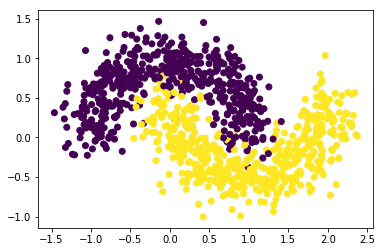
Two-Moons Classification
We use the classic two-moons dataset, consisting of two interleaving half circles with added noise, in order to test and compare classification results for AdaBoost and Gradient Boosting (see below). This dataset is conveniently built-in to scikit-learn and accessible via make_moons, which returns a data matrix X and a label vector y. We can treat the dataset as a complete training set as we eventually use cross-validation to estimate the test error.
from sklearn.ensemble import AdaBoostClassifier
from sklearn.tree import DecisionTreeClassifier
import numpy as np
import matplotlib.pyplot as plt
%matplotlib inline
from sklearn.datasets import make_moons
N = 1000
X,Y = make_moons(N,noise=0.2)
plt.scatter(X[:,0],X[:,1], c=Y)
plt.show()
We first try to classify the data using a decision tree using DecisionTreeClassifier with maximum depth of 3 (this structure will later be used for our weak learners).
clf = DecisionTreeClassifier(max_depth=3)
clf.fit(X,Y)
xx,yy = np.meshgrid(np.linspace(-1.5,2.5,50),np.linspace(-1,1.5,50))
Z = clf.predict(np.c_[xx.ravel(), yy.ravel()])
Z = Z.reshape(xx.shape)
plt.scatter(X[:,0],X[:,1], c = Y)
plt.contourf(xx,yy,Z,alpha=0.3)
plt.show()
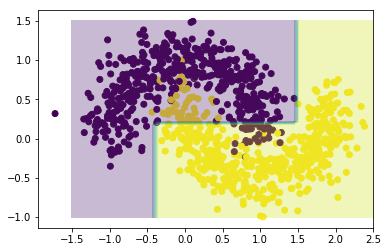
As can be seen from the graph above, this single decision tree does not provide the best of fits.
Next, we obtain an AdaBoost classification. Let’s first consider a model consisting of 10 decision trees, and with a learning rate of 1/10.
ada = AdaBoostClassifier(clf, n_estimators=10, learning_rate=0.1)
ada.fit(X,Y)
xx,yy = np.meshgrid(np.linspace(-1.5,2.5,50),np.linspace(-1,1.5,50))
Z = ada.predict(np.c_[xx.ravel(), yy.ravel()])
Z = Z.reshape(xx.shape)
plt.scatter(X[:,0],X[:,1], c = Y)
plt.contourf(xx,yy,Z,alpha=0.3)
plt.show()
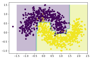
The AdaBoosted tree is better at capturing the dataset’s structure. Of course, until we evaluate the performance on an independent test set, this could simply be a consequence of overfitting (one of AdaBoost’s main weaknesses, as the procedure is sensitive to outliers and noise). We can guard against this eventuality by adjusting the learning rate (which provides a step size for the algorithm’s iterations).
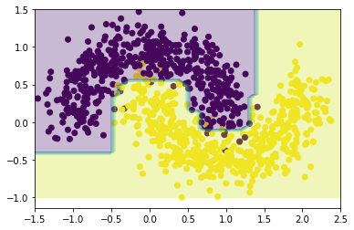
To find the optimal value for the learning rate and the number of estimators, one can use the GridSearchCV method from sklearn.model_selection, which implements cross-validation on a grid of parameters. It can also be parallelized, in case the efficiency of the algorithm should ever need improving (that is not necessary on such a small dataset, but could prove useful with larger datasets).
from sklearn.model_selection import GridSearchCV
params = {
     'n_estimators': np.arange(10,300,10),
     'learning_rate': [0.01, 0.05, 0.1, 1],
 }
grid_cv = GridSearchCV(AdaBoostClassifier(), param_grid= params, cv=5, n_jobs=-1)
grid_cv.fit(X,Y)
grid_cv.best_params_
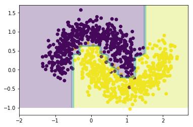
{'learning_rate': 0.05, 'n_estimators': 230}The results show that, given the selected grid search ranges, the optimal parameters (those that provide the best cross-validation fit for the data) are 230 estimators with a learning rate of 0.05. The plot of the model of these parameters indeed shows that the fit looks might fine.
ada = grid_cv.best_estimator_
xx,yy = np.meshgrid(np.linspace(-1.5,2.5,50),np.linspace(-1,1.5,50))
Z = ada.predict(np.c_[xx.ravel(), yy.ravel()])
Z = Z.reshape(xx.shape)
plt.scatter(X[:,0],X[:,1], c = Y)
plt.contourf(xx,yy,Z,alpha=0.3)
plt.show()
Gradient Boosting
The implementation of Gradient Boosting is simpler than AdaBoost. The idea is to first fit a model, then to compute the residual generated by this model. Next, a new model is trained, but on the residuals instead of on the original response. The resulting model is added to the first one. Those steps are repeated a sufficient number of times. The final model will be a sum of the initial model and of the subsequent models trained on the chain of residuals.
In theory, the Gradient Boosted model solves (with the notation used for AdaBoost above)


where  are weak learners for . The final gradient boosted learner is
  . The choice of the appropriate loss function
  depends on the nature of the supervised learning task. In practice, the solution must be approximated with a steepest (gradient) descent method (whence the name Gradient Boosting).
When the weak learners are decision trees, the in the formulation above can be re-written as
![\[f_m(\vec{x})=\sum_{j=1}^{J_m}b_{j,m} \chi_{R_{j,m}}(\vec{x}),\]](https://www.data-action-lab.com/wp-content/ql-cache/quicklatex.com-f0a99c2de37a2a063a59b5b4fb364c2f_l3.png "Rendered by QuickLaTeX.com")
 is the characteristic function on the subregion
  of the predictor space:
 ![\[\chi_{R_{j,m}}(\vec{x})=\begin{cases}1 \text{ if }\vec{x}\in R_{j,m} \\ 0 \text{ otherwise}\end{cases}\]](https://www.data-action-lab.com/wp-content/ql-cache/quicklatex.com-b5e37b4d0f9695b05aed65b2d997c243_l3.png "Rendered by QuickLaTeX.com")
partitions the predictor space into  disjoint regions
  .
.
In that case, Friedman (1999) suggests a modification to the original problem that eliminates the coefficients  in the definition of , and produces a simpler rule to update the model (TreeBoost):


The depth of the weak learners (the ) can be adjusted to vary between stumps ( ) to interaction models (
 ); there is evidence to suggest that
  is adequate for most boosting applications (see Wikipedia).
Implementation
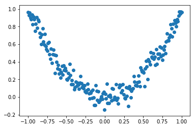
Consider a simple implementation of Gradient Boosting on a training set consisting of a noisy parabola.
N = 200
X = np.linspace(-1,1,N)
Y = X**2+ np.random.normal(0,0.07,N)
X = X.reshape(-1,1)
plt.scatter(X,Y)
plt.show()
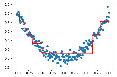
With this data, we can use DecisionTreeRegressor from sklearn.tree to fit the initial model F_0.
from sklearn.tree import DecisionTreeRegressor
reg1 = DecisionTreeRegressor(max_depth=3)
reg1.fit(X,Y)
plt.figure()
plt.scatter(X,Y)
plt.plot(X,reg1.predict(X), 'r')
plt.show()
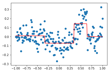
We can now compute the residuals and fit a new model f_0 on it.
Y2 = Y - reg1.predict(X)
reg2 = DecisionTreeRegressor(max_depth=2)
reg2.fit(X,Y2)
plt.scatter(X,Y2)
plt.plot(X,reg2.predict(X),'r')
plt.show()
The resulting model at this step is F_1 = F_0 + f_0.
F_0 = reg1.predict(X)
f_0 = reg2.predict(X)
F_1 = F_0 + f_0
plt.scatter(X,Y)
plt.plot(X,F_1,'r', label = "F_0 + f_0")
plt.plot(X,F_0,'g', label = "F_0")
plt.legend()
plt.show()
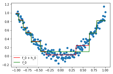
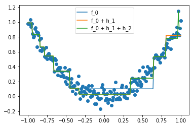
Here, we can see that the new model F_1 (in red) is a better fit for the data than F_0 (in green). Reaping this process a second time, we get an even better approximation F_2.
Y3 = Y2 - reg2.predict(X)
reg3 = DecisionTreeRegressor(max_depth=2)
reg3.fit(X,Y3)
f = sum(tree.predict(X) for tree in (reg2,reg3))
F_2 = F_0 + f
plt.scatter(X,Y)
plt.plot(X,F_0, label = "F_0")
plt.plot(X,F_1, label = "F_0 + f_1")
plt.plot(X,F_2, label = "F_0 + f_1 + f_2")
plt.legend()
plt.show()
Doing this manually can be tedious, so we use GradientBoostingRegressor from sklearn.ensemble, which recreates the steps we’ve produced above.
from sklearn.ensemble import GradientBoostingRegressor
from sklearn.metrics import mean_squared_error as mse
fig=plt.figure(figsize=(12, 8), dpi= 80, facecolor='w', edgecolor='k')
for n in enumerate([1,3,5,10]):
    gb = GradientBoostingRegressor(max_depth=2, n_estimators=n[1],learning_rate=1)
    gb.fit(X,Y)
    plt.subplot(2,2,n[0]+1)
    plt.scatter(X,Y)
    plt.plot(X,gb.predict(X), 'r')
    acc = mse(Y, gb.predict(X))
    plt.title('n = %i, mse = %f' %(n[1], acc))
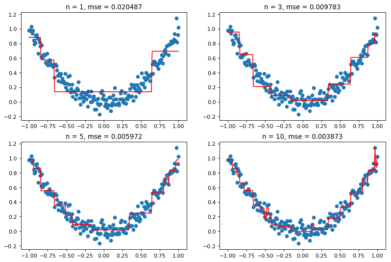
As we can see from the figure above, increasing the number of steps leads to a better fit, and thus to a lower mean squared error (MSE). However, this may also lead to overfitting, which is why this parameter should not be too high. There are many ways to determine the optimal for a given dataset; cross-validation (as we did for AdaBoost above) is a commonly-used approach.
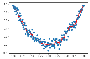
params = {
     'n_estimators': np.arange(1,101),
     'learning_rate': [0.01, 0.05, 0.1, 1],
 }
grid_cv = GridSearchCV(GradientBoostingRegressor(max_depth=2), param_grid= params, cv=5, n_jobs=-1)
grid_cv.fit(X,Y)
print("Best params:", grid_cv.best_params_)
clf = grid_cv.best_estimator_
plt.scatter(X,Y)
plt.plot(X,clf.predict(X), 'r')
plt.show()
Classification
With the appropriate loss function, Gradient Boosting also works for classification. Here’s a simple example, using the data generated by the make_moons function from sklearn.dataset.
N = 1000
X,Y = make_moons(N,noise=0.2)
gbc = GradientBoostingClassifier(n_estimators=9, learning_rate=0.5)
gbc.fit(X,Y)
xx,yy = np.meshgrid(np.linspace(-1.5,2.5,50),np.linspace(-1,1.5,50))
Z = gbc.predict(np.c_[xx.ravel(), yy.ravel()])
Z = Z.reshape(xx.shape)
plt.scatter(X[:,0],X[:,1], c = Y)
plt.contourf(xx,yy,Z,alpha=0.3)
plt.show()
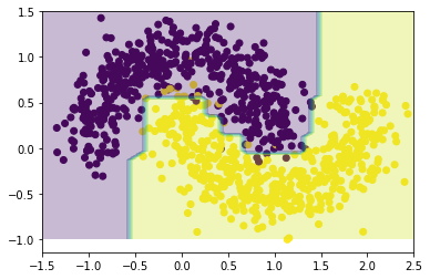
from sklearn.metrics import accuracy_score
accuracy_score(y_pred=gbc.predict(X), y_true=Y)
0.985We can see that the resulting model has a pretty good accuracy as well (although the value on its own is meaningless as without some evaluation of the test error).
XGBoost
<code>XGBoost</code> is a popular library that implement Gradient Boosting. It also implements Stochastic Gradient Boosting and Regularized Gradient Boosting (popular variants of Gradient Boosting) and features parallelization, distributed computing, out-of-core computing and cache optimization, and a built-in missing value handler. All those features make <code>XGBoost</code> fast and flexible, which explains why it has been used by many competitors in the various Kaggle contests.
Here is the same two-moons classification example, but tackled by <code>XGBoost</code>.
from xgboost import XGBClassifier
N = 1000
X,Y = make_moons(N,noise=0.2)
xgb = XGBClassifier(reg_alpha=1, reg_lambda=0)
xgb.fit(X,Y)
xx,yy = np.meshgrid(np.linspace(-2,2.7,50),np.linspace(-1,1.7,50))
Z = xgb.predict(np.c_[xx.ravel(), yy.ravel()])
Z = Z.reshape(xx.shape)
plt.scatter(X[:,0],X[:,1], c = Y)
plt.contourf(xx,yy,Z,alpha=0.3)
print("Accuray: ",accuracy_score(y_pred=xgb.predict(X), y_true=Y))
Accuray: 0.989
Without much configuration of the parameters, other than imposing a L1 regularization on the weights, <code>XGBoost</code> performs very well on this toy example.
Comparison and Performance
Let’s use another built-in dataset to compare the performance of AdaBoost, Gradient Boosting, and Regularized Gradient Boosting. We use the Wisconsin Breast Cancer Diagnostic dataset (Wolberg, Street, Mangasarian, 1995), which consists of 30 features and a diagnosis with 2 labels (see UCI Machine Learning Repository).
Attributes Information:
- radius (mean of distances from center to points on the perimeter)
- texture (standard deviation of gray-scale values)
- perimeter
- area
- smoothness (local variation in radius lengths)
- compactness (perimeter^2 / area – 1.0)
- concavity (severity of concave portions of the contour)
- concave points (number of concave portions of the contour)
- symmetry
- fractal dimension (“coastline approximation” – 1)
The mean, standard error, and “worst” or largest (mean of the three largest values) of these features were computed for each image, resulting in 30 features. Features are computed from a digitized image of a fine needle aspirate (FNA) of a breast mass. They describe characteristics of the cell nuclei present in the image.
The goal is to use those features to classify each tumor to one of two labels: Malignant (1) or Benign (0).
The data is split into a training and a testing set, to test the models on instances which are independent from the observations with which they were trained. Each model were then fitted using optimal algorithm parameters, found via cross-validation.
from sklearn.datasets import load_breast_cancer
from sklearn.model_selection import train_test_split
from time import time
X,y = load_breast_cancer(return_X_y=True)
X_train, X_test, y_train, y_test = train_test_split(X,y)

xgb = XGBClassifier(eta = 0.01, max_depth=4)
t0 = time()
xgb.fit(X_train,y_train)
t1 = time()
print("XGBoost:","Time =",t1-t0, "Accuracy =", accuracy_score(y_pred = xgb.predict(X_test), y_true=y_test))
gbc = GradientBoostingClassifier(max_depth=3, n_estimators=67, learning_rate=0.1)
t0 = time()
gbc.fit(X_train,y_train)
t1 = time()
print("GradBoost:","Time =",t1-t0, "Accuracy =", accuracy_score(y_pred = gbc.predict(X_test), y_true=y_test))
clf = DecisionTreeClassifier(max_depth=3)
ada = AdaBoostClassifier(clf,n_estimators=155, learning_rate=0.5)
t0 = time()
ada.fit(X_train,y_train)
t1 = time()
print("AdaBoost:","Time =",t1-t0, "Accuracy =", accuracy_score(y_pred = ada.predict(X_test), y_true=y_test))
| Algorithm | Time (s) | Accuracy |
| XGBoost | 0.1435 | 0.972 |
| Gradient Tree Boosting | 0.1356 | 0.965 |
| Adaboost with Tree | 0.7316 | 0.965 |
As we can see, all models perform roughly at the same level, but AdaBoost (with decision trees) is substantially slower than then other two models.